CSIRO Computing History Appendix 7: CSIRO Computing Museum / Artefacts
This page/post is continuing to be constructed.
Last updated: 21 Dec 2023.
Updated locations of saved material.
Robert C. Bell
Appendix 6 — Computing History Home — Appendix 8
This is the start of a CSIRO on-line Computing Museum with images of a collection of artefacts.
- Sample punched cards, contained in a standard cardboard box that cards were packaged in.

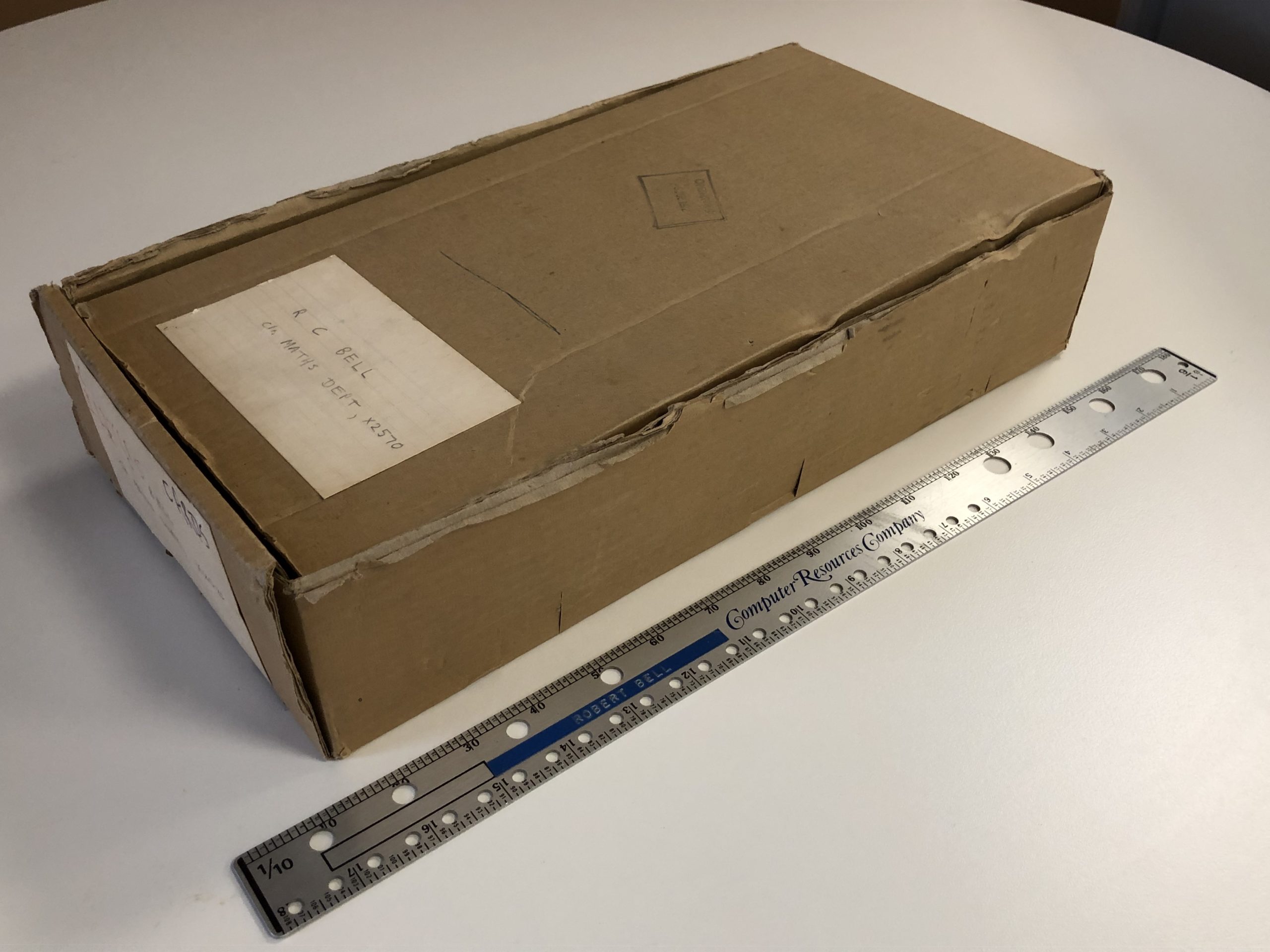
Here’s the box, with an 18″ (450mm) ruler beside it to give some scale. The following shows the contents of the box – mostly punched cards, but there is some paper tape, a 3 1/2″ floppy disc (from a later era), and a write-ring.
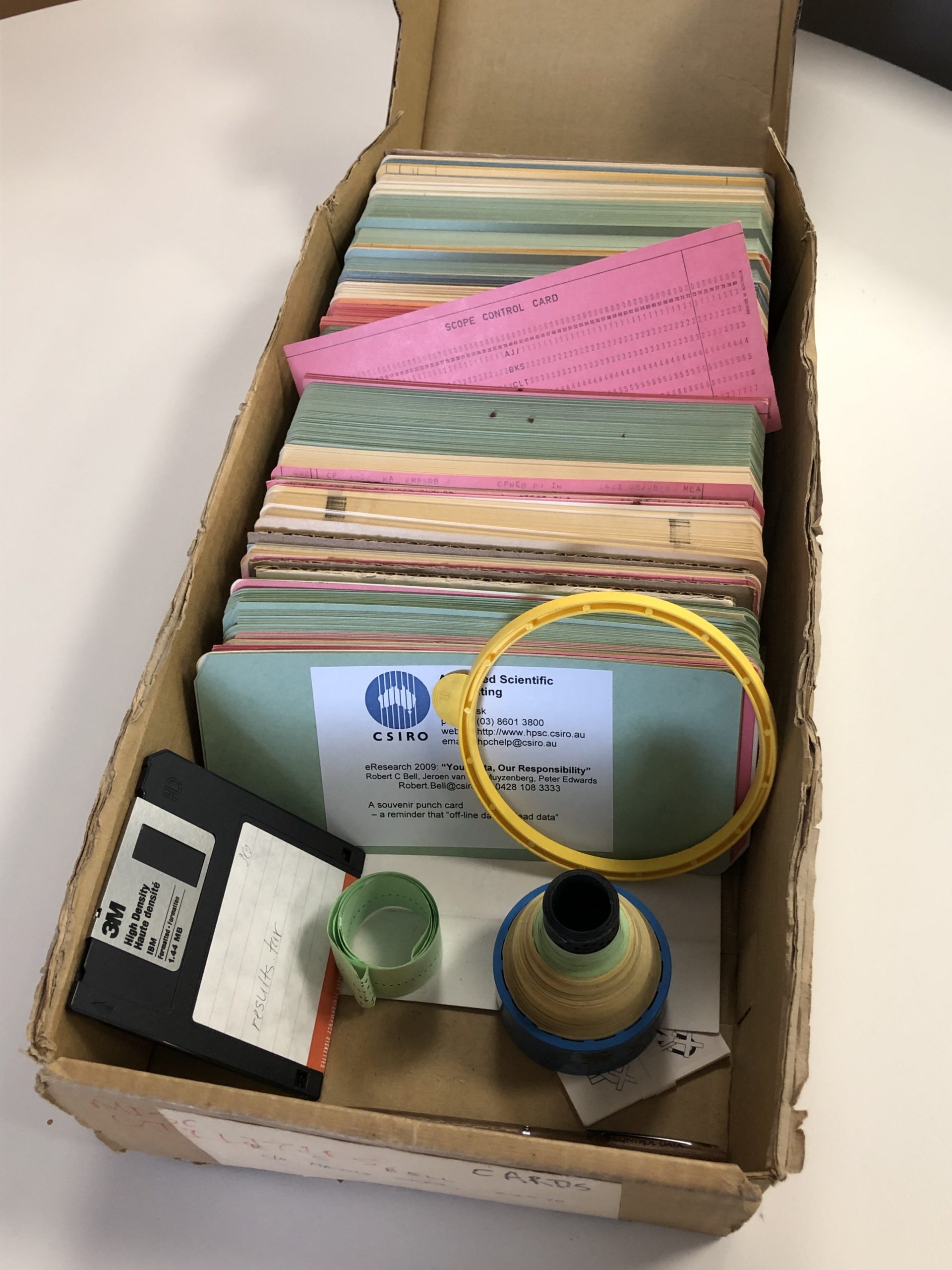
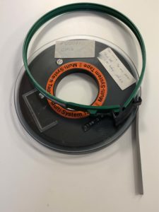
A write-ring came with every (round) magnetic tape. It could be inserted in a circular groove on the back of a tape. If it was present, the tape drive could sense it, and would allow writing on the tape. If it was not present, the drive would allow only reading. Of course, you only needed one write-ring per drive, but one came with every tape, so they were plentiful. I don’t think anyone found a good use for the excess!
The pink card was a SCOPE Control Card used on either the Monash CDC 3200 – it was the second card in a deck after the yellow sequence card, or on the CDC Cyber 76, and contained the job name, charge code, and resource requests.
Here’s another picture of paper tape – this one was to be used for Christmas decorations, not data input!

2. Sample magnetic tapes/cartridges/write-ring
The first picture shows a magnetic tape dating from about 1990. It belonged to the Division of Atmospheric Research, and contained files from the end of CSIRO’s usage of Csironet. The tape was 9-track, and probably 6250 bits per inch, and could store about 150 Mbyte on the 2400 foot length.
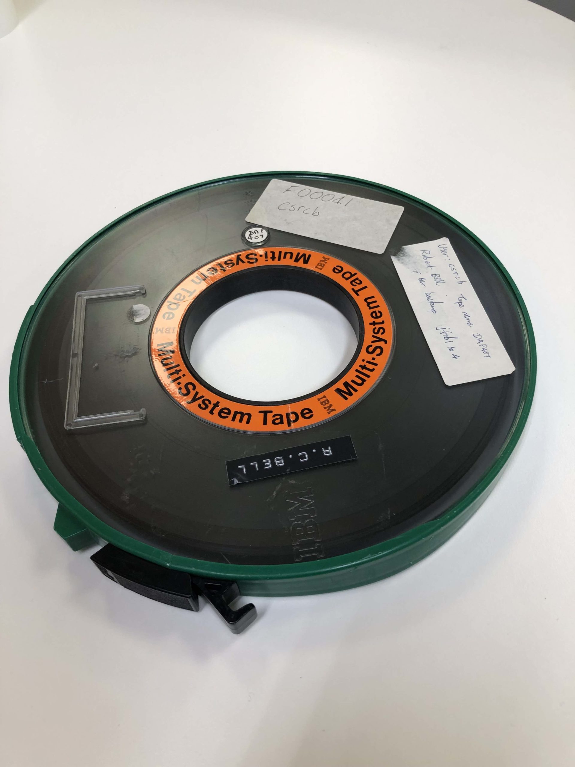
The second image shows the back of the tape with a write-ring in place. The tape drives had a retractable pin which sensed the presence of the ring or not.
The third image shows the tape with the protective cover removed. This one did not have the small holes in it which some drives could use to remove the protective cover by forcing air through the holes. The end of the 1/2-inch width tape is shown. I didn’t find the reflective marker which showed the beginning of the information, and was used by the drives to trigger reading of the tape, but probably didn’t look far enough down the tape.
High speed tape drives such as those shown in the image for Chapter 2 had vacuum loops either side of the read/write heads, so that the tape could be stopped and started suddenly without breaking the tape. When tapes were re-wound, this could be done at high speed, and the noise was like a jet engine.
3. Sample coding forms
Coding forms were pads of pre-printed stationery, used by programmers to write out their programs, or by data-entry staff to enter data extracted from elsewhere. From there, coding forms were passed to ‘punch-girls’ (sorry, that was the name used) who keyed the data into a card punch (typically an IBM 26 or 029 punch) which produced punched cards. Punched cards were read by card readers attached to the computers, and cards were the primary input media.
The first example is a CDC Fortran coding sheet, showing the various reserved fields (e.g. Type, statement number, continuation, statement and serial number). These cards were processed by the Fortran compiler. The second is a CDC data sheet.
The third is a CSIRO Data Sheet, with the cards typically used as input to programs.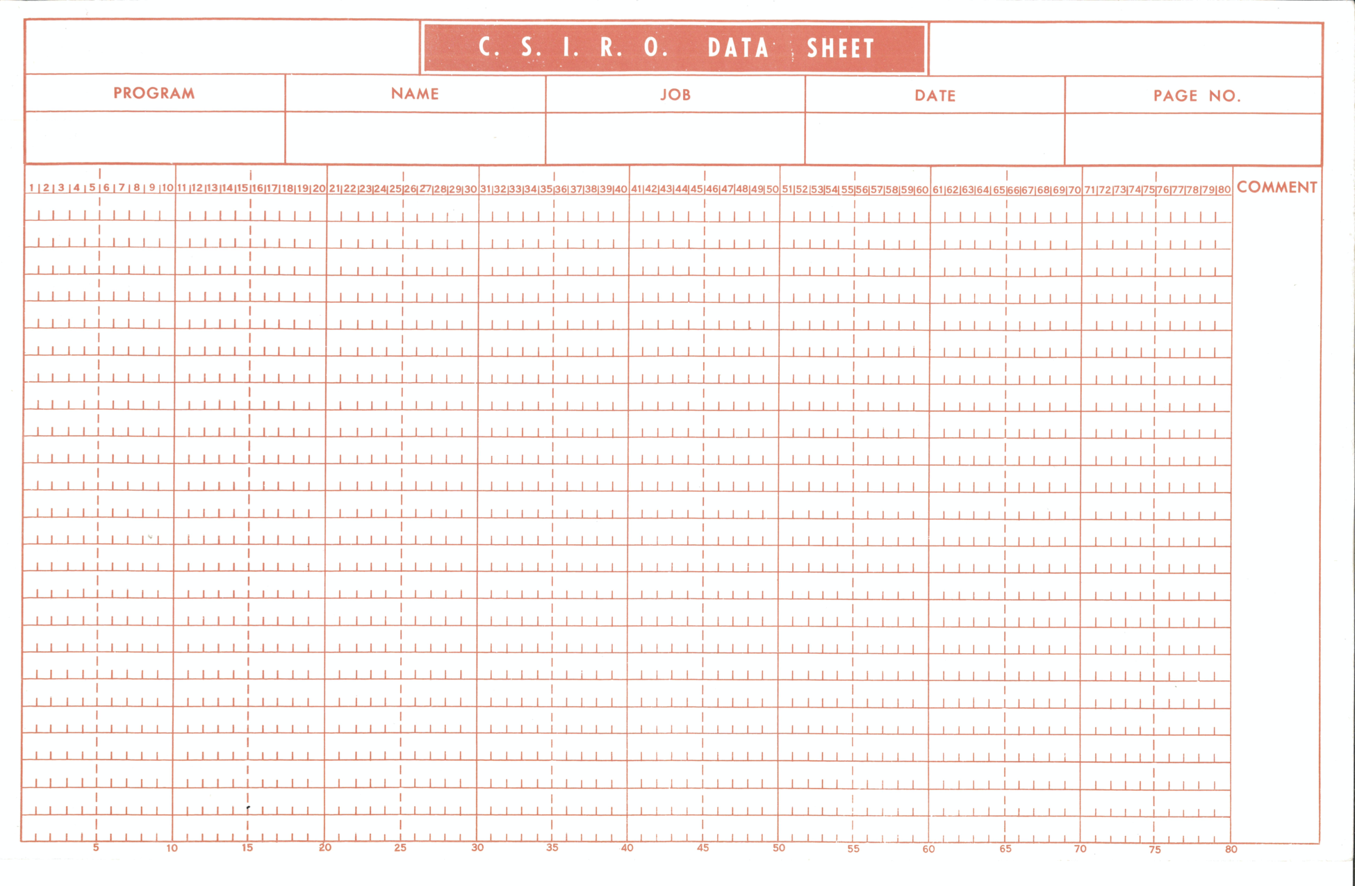
The fourth is a Rob. Bell attempt to provide cheaper and more readable coding forms. Students couldn’t afford coding sheets, nor did they have access to the dedicated card punch operators, so used any available paper.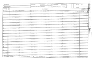
The fifth is a Bureau of Meteorology IBM System / 360 Fortran Coding Form. This one was bigger than the CDC one.
Note that the Fortran coding forms had special instructions about the representation of letters and digits that could be easily confused, especially if the card punch operators had no context to help. For example, there might be a line
120 DO 1200 I1 = IO, IZ, 2
and most of the spaces could legally be squeezed out:
120 DO1200I1=I0,IZ,2
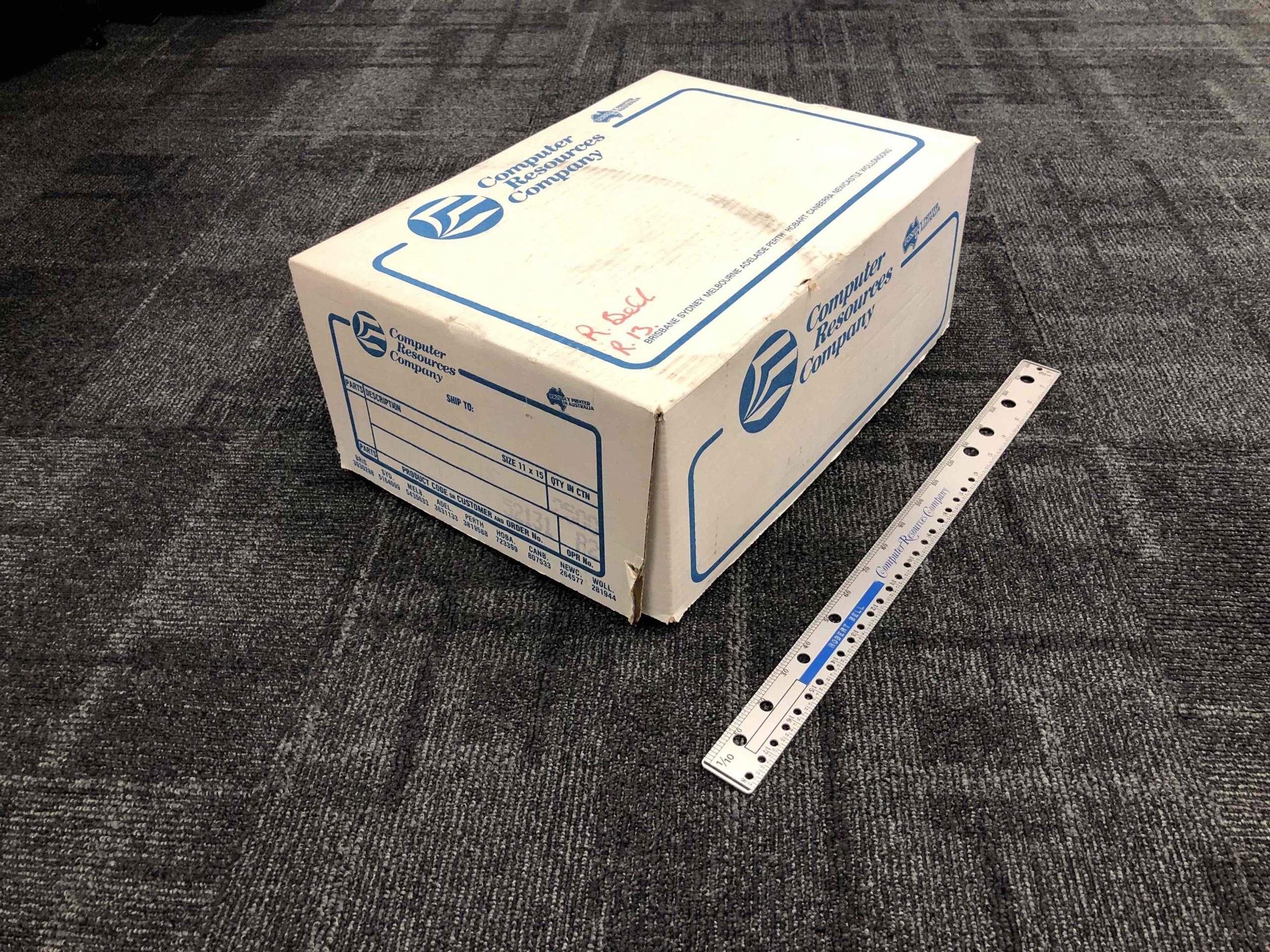
4. Special ruler for use with 11” x 15” paper
(See section 31 below).
5. Printed 11″ x 15″ output (see item 32. below), and boxes in which this paper was delivered (The faint print on the side of the box showed that it held 2500 sheets.)
 The paper was fan-folded (Z-fold), had sprocket holes down each side, and was printed by line printers with print drums (which pre-dated dot-matrix and other printers – see Wikipedia ). Line printers were capable of printing up to about 1200 lines per minute, and were extremely noisy.
When DCR moved to acquire a Computer Output Microfilm (COM) system, it reported that “Microfiche saves printing time/costs: total printing about 140,000 pages per day (56 boxes!)”.
(DCR Newsletter no. 129, Sep 1976). Each box weighed around 20 kg, so over 1 tonne of paper per day was being consumed!
Wikipedia: The names of the lp and lpr commands in Unix were derived from the term “line printer”.
The coming of computer printing led to a revolution in kindergartens and schools – the wide availability of paper. Scrap paper was plentiful, and found its way into homes and then to kindergartens and schools. Many first paintings were done on the back of printouts. Printed output from organisations like CSIRO rarely had security implications (apart from payroll runs!), and so could be safely reused. What was especially prized was blank paper. When a printer finished a printout, there was usually another following, and the operators were responsible for tearing the paper between each output. When there was no following output, it was simple to press a button to take the printer off-line, press another button to eject a page or two, collect the printout, and then press the button again to put the printer on-line. This left 2 or 3 blank pages at the beginning of the next printout. Of course, it could be terribly noisy to stick your head down behind a a printer in action – we measured over 100 decibels behind a printer at Aspendale.
6. Flowchart template
(See section 31 below).
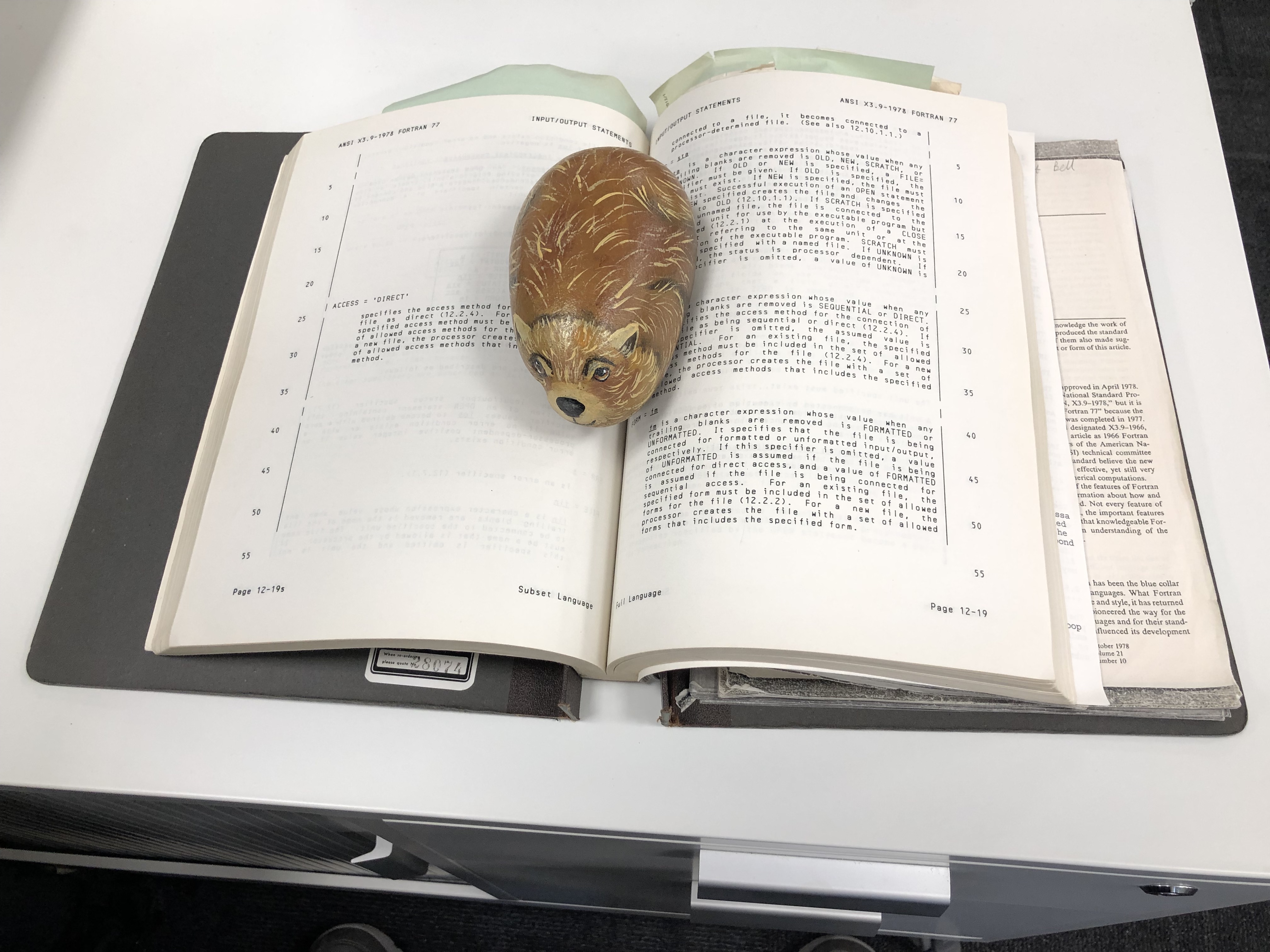
7. Rock and three-ringed binders
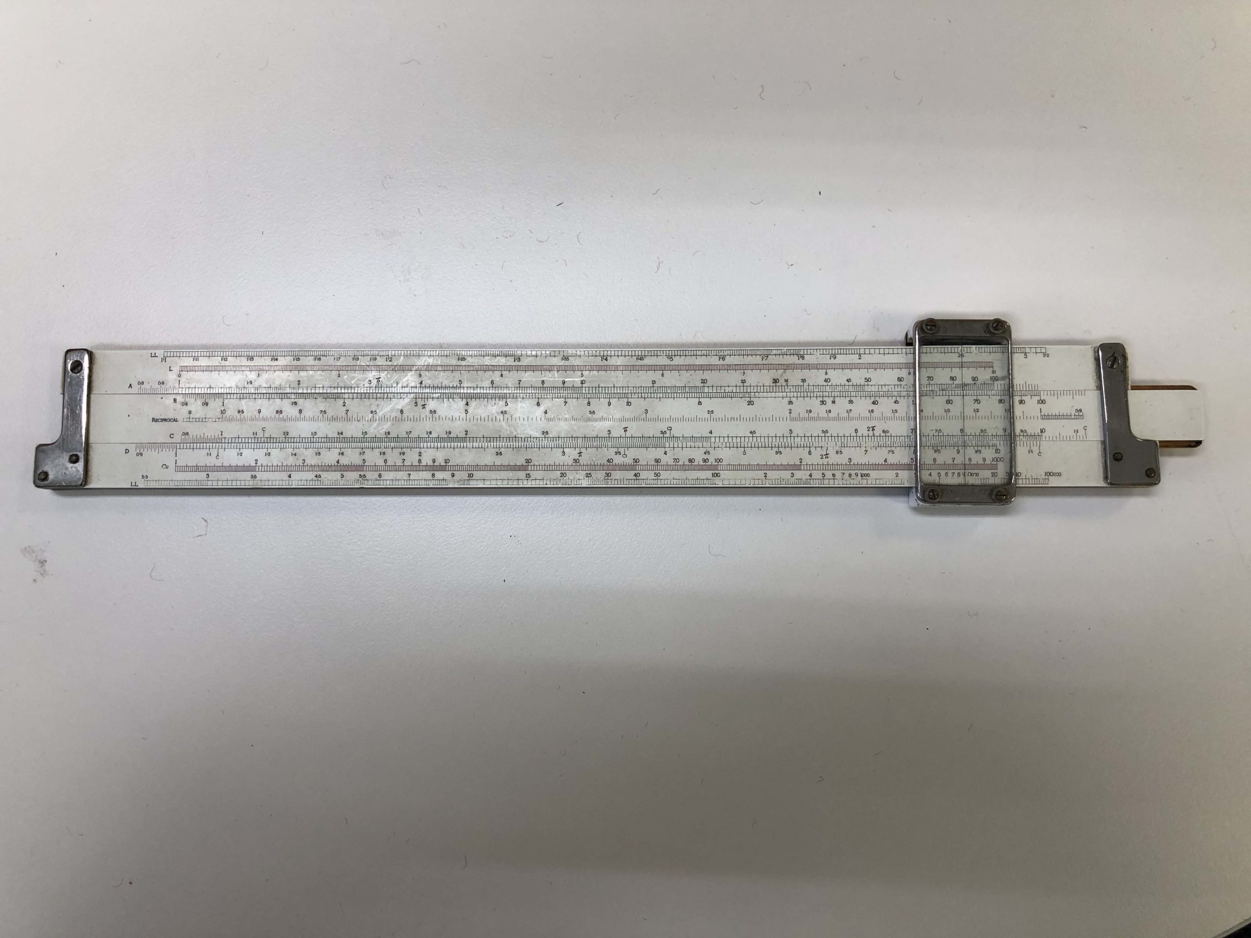
8. Slide rule
A slide rule is one of the earliest analog computing devices: especially favoured by engineers. It was ideal for multiplying numbers with up to 3 significant figures.
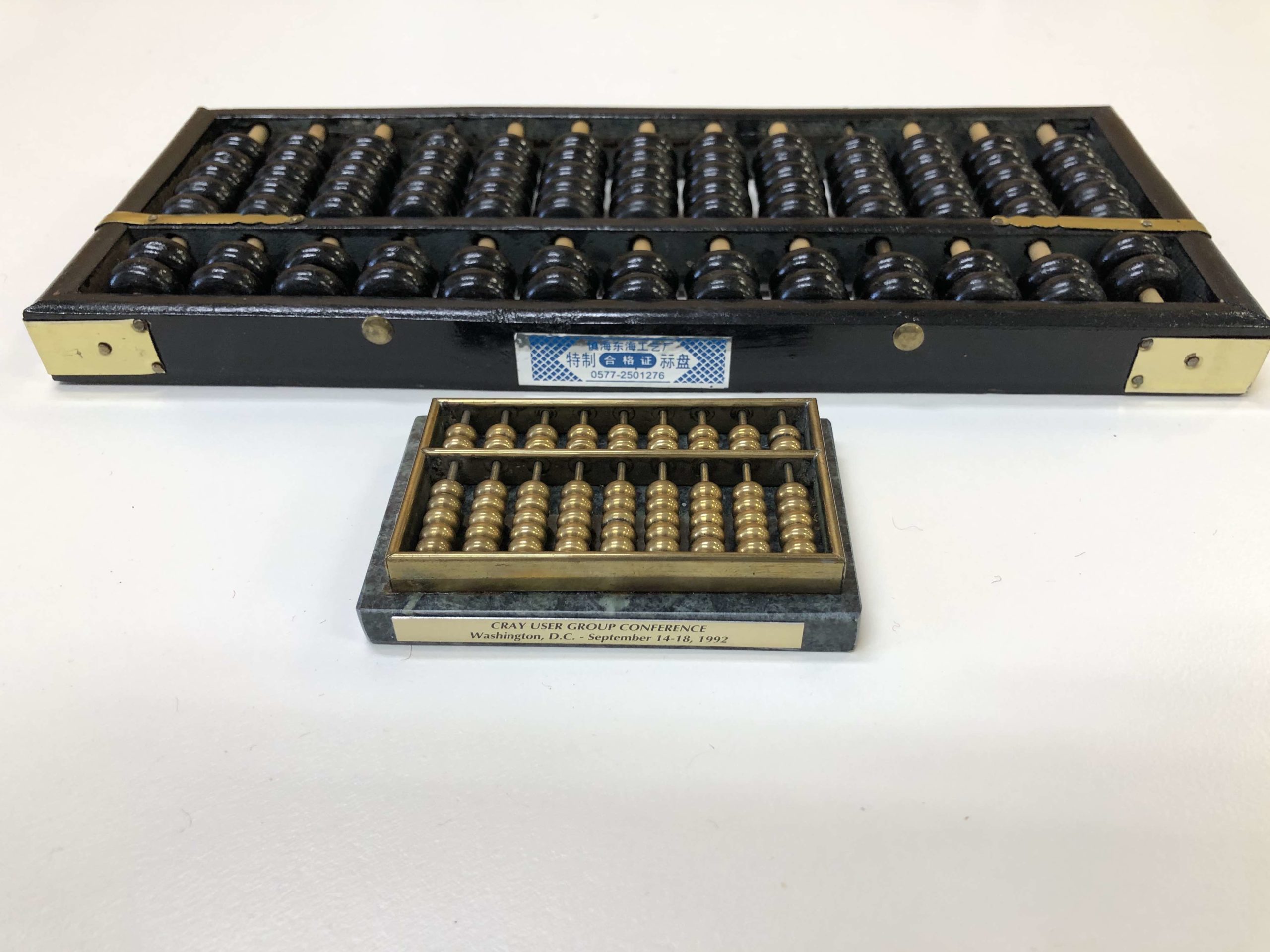
9. Abacus (small and large)
These were favoured for financial calculations. The small one is a souvenir from the Cray User Group.
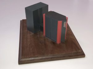
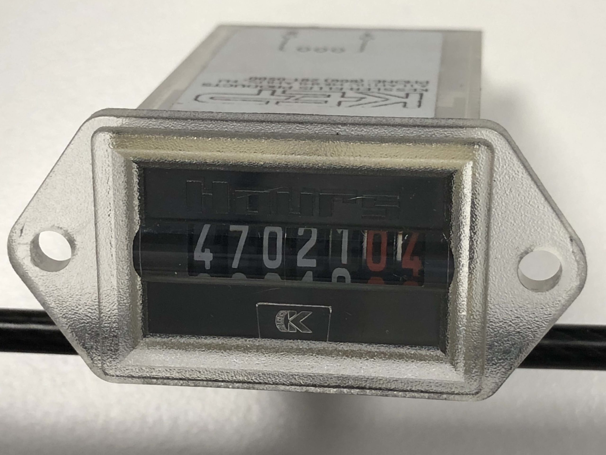
10. Model of a Cray Research Y-MP 4E supercomputer, the centrepiece of the CSIRO Supercomputing Facility, hosted at the University of Melbourne from 1992 to 1997 in the Thomas Cherry Building. In the machine room were the major University systems, including a CDC Cyber 990, and the ACCI IBM 3090 VF, alongside SN 1918, the Y-MP. See Chapter 6 of the CSIRO Computing History for further details, including a picture of the actual system. A brochure on the Y-MP4E is held by Rob Bell, and is available on-line here.
 Here is a photo of the counter showing the number of hours used from SN 1918 – 47021.04 hours – over 5 years.
11. Cray Y-MP4 front panel
12. Cray Y-MP CPU (costing about $250k around 1995)
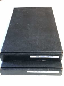
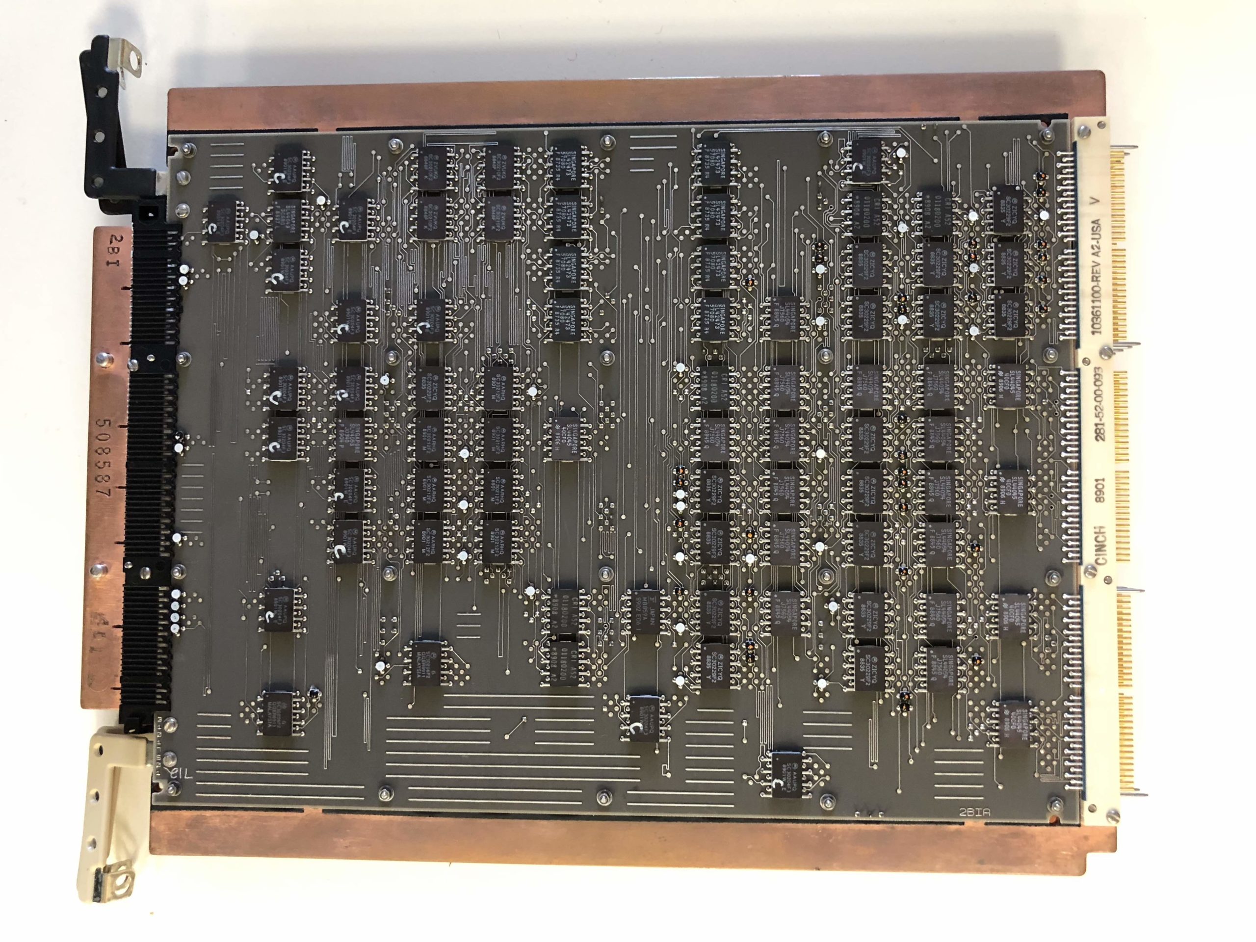
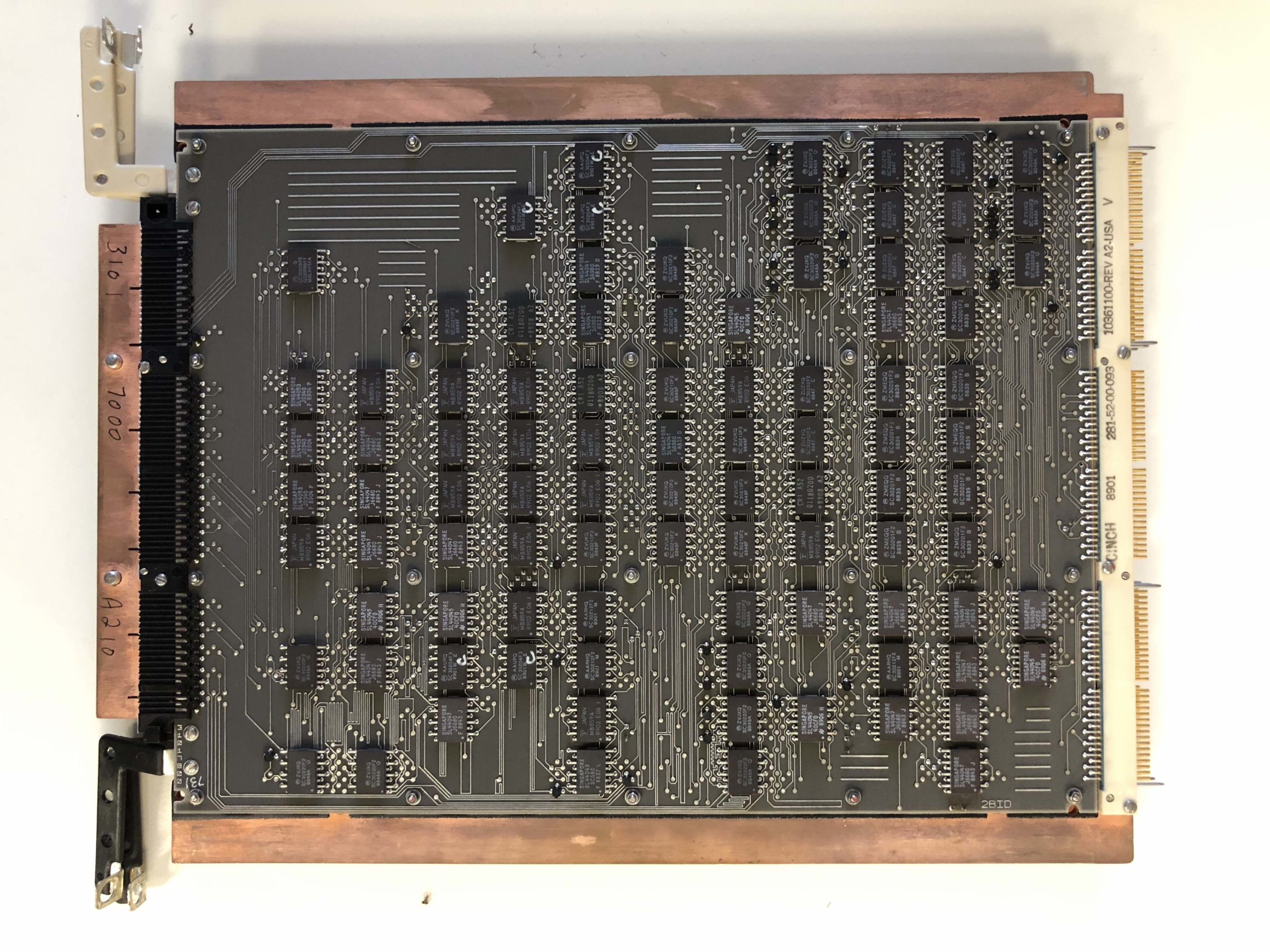
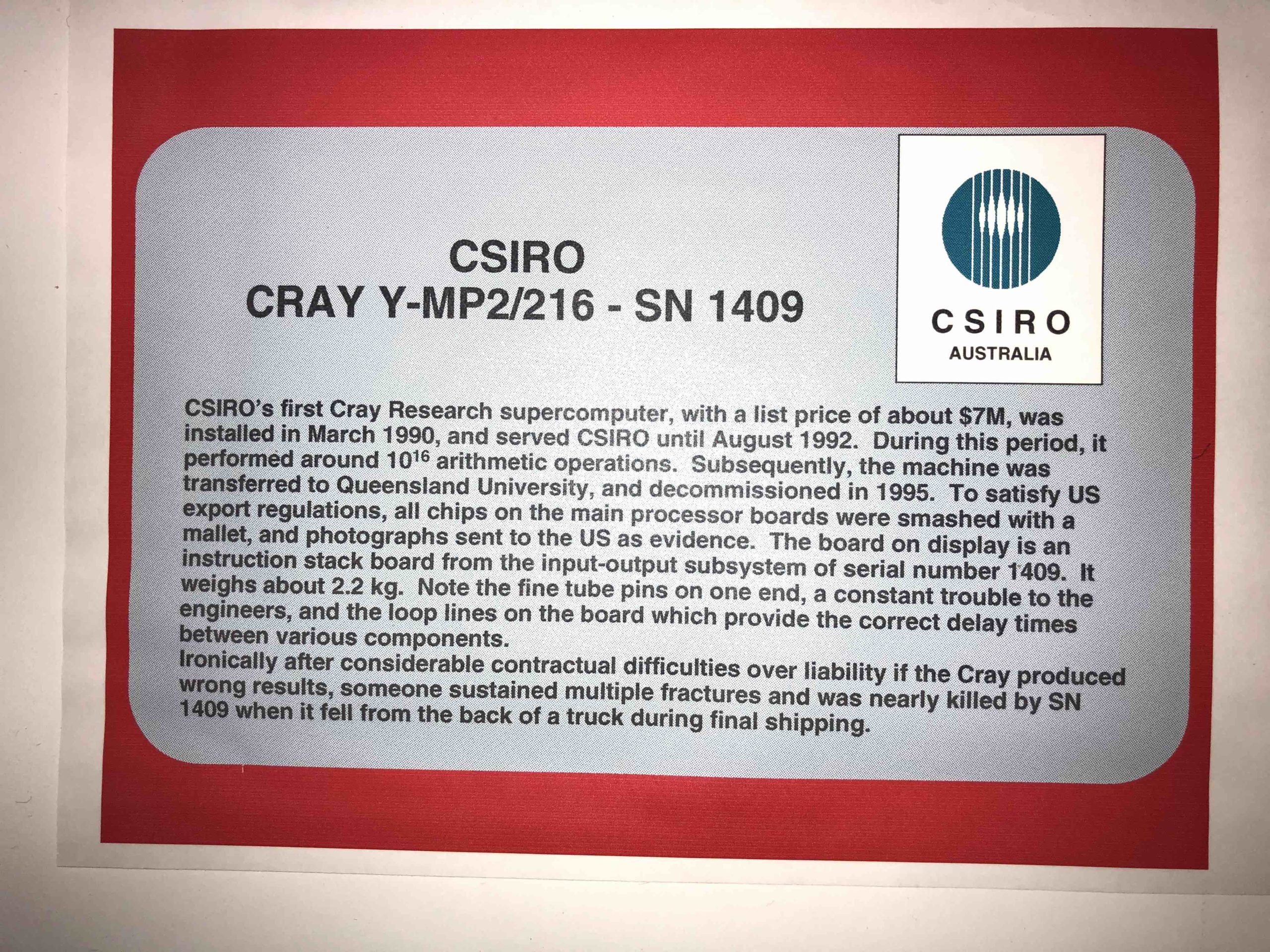
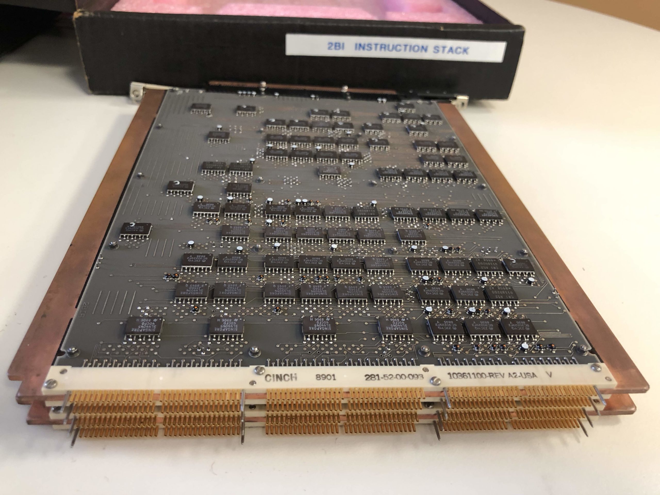
13. Circuit boards from Cray Y-MP2/216 SN 1409 IOS – Cray X-MP technology
The first CSIRO Cray Y-MP used predecessor X-MP technology for the input/output subsystem. These two boxes contain two boards from the IOS – a very high speed channel controller, and an instruction stack board.
 Inside each box is a board, packed in foam.
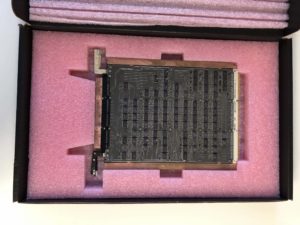
Here’s one side of a board:
 Here’s a description written in the early 21st century:
This shot shows the gold tubes on the end of the board:
Here’s a close-up: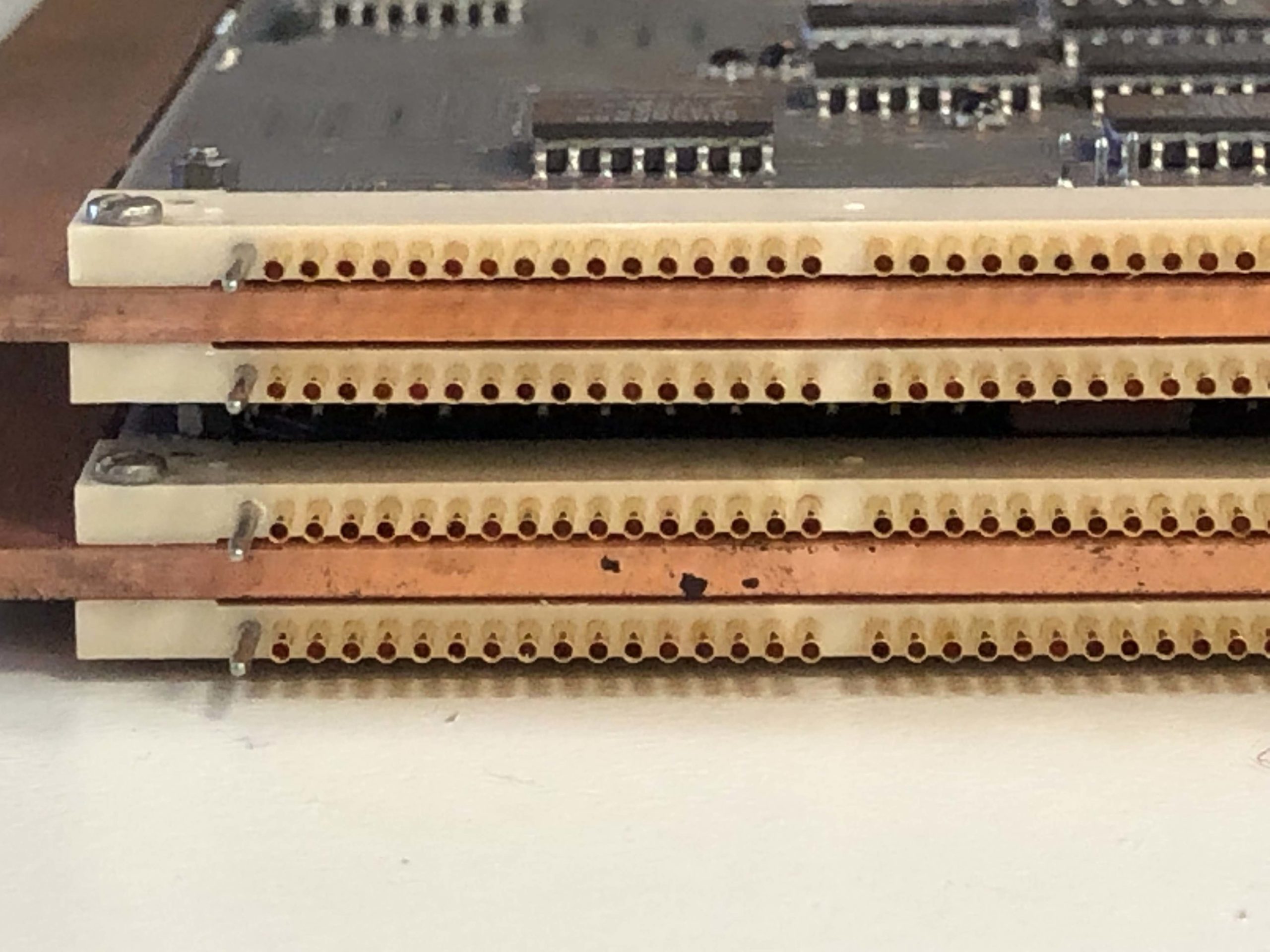
These tubes were reported to be a nightmare by the engineers – one bent pin meant the board was a write-off: being made of gold, the pins were malleable.
14. Cray J90se CPU board
15. CPU from NEC SX-6
16. Commemorative book of the build of Cray Y-MP2/216 SN 1409
17. CDC Manuals – complete set of user manuals from 1985 for the CDC Cyber 76 (SCOPE 2)
18. CDC Manuals – complete set of user manuals from 1990 for the CDC Cyber 205 (VSOS)
19. CRS/DCR/Csironet News – complete set
20. DCR/Csironet Cybarites – technical newsletter
21. DCR/Csironet Staff News
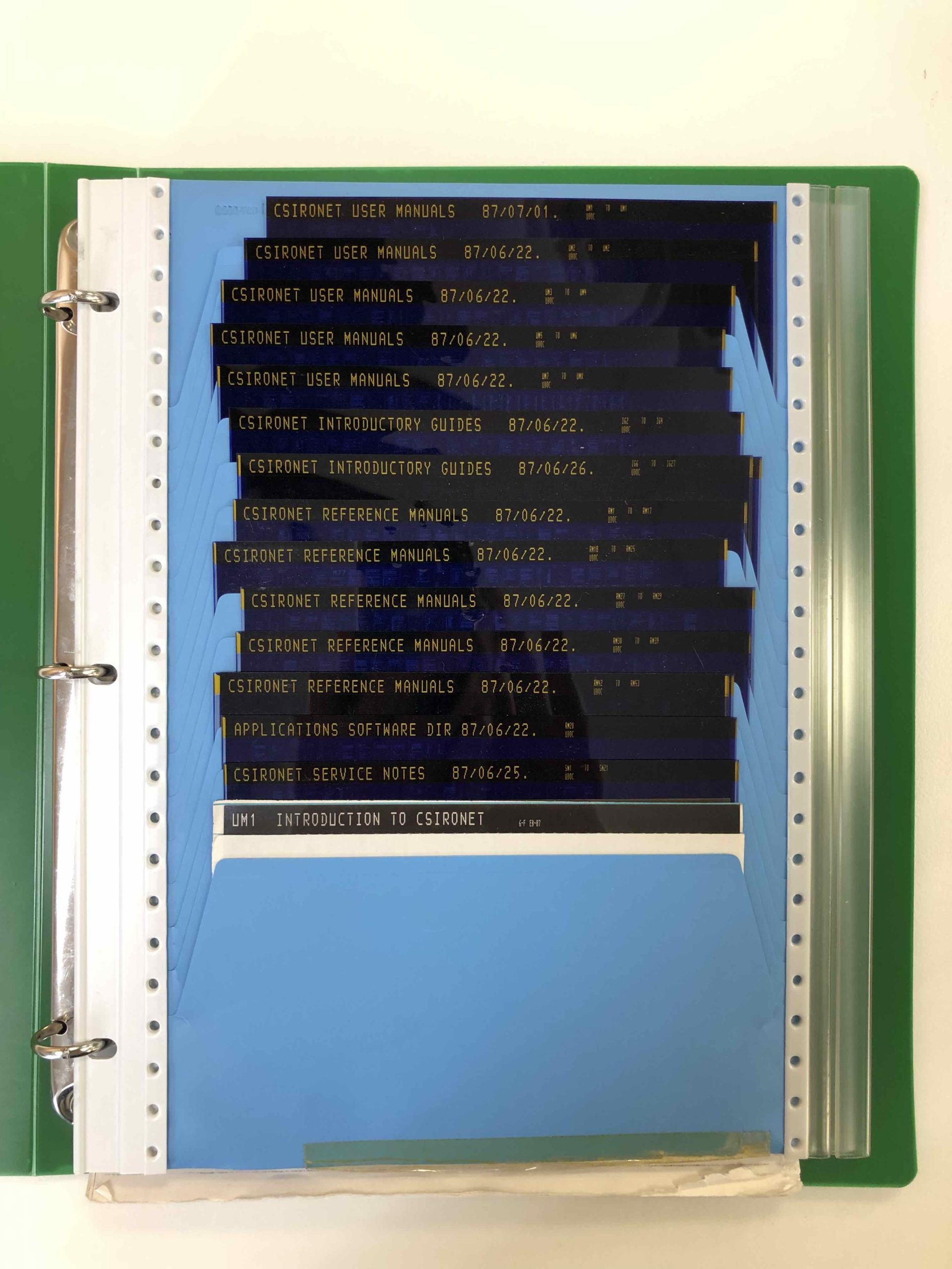
22. Microfiche – Csironet manuals
Here are some pictures of microfiche – firstly, a 3-ringer binder holder, with the entire Csironet user documentation: then two microfiche – the black one is an original, the blue one a copy. Up to 420 quarto pages and 280 line-printer page images could be written on each microfiche.
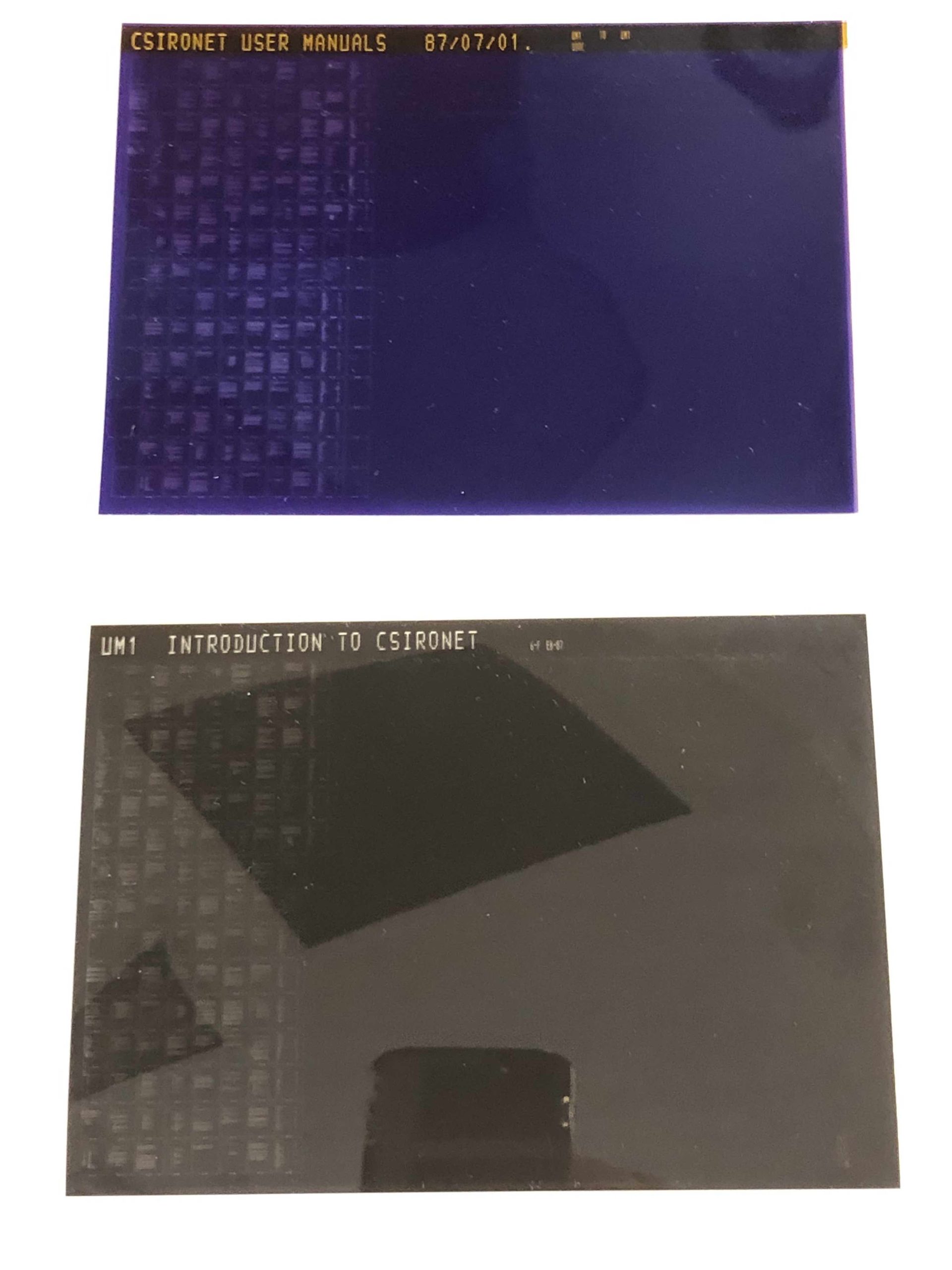 (The shapes in the second image are reflections, not on the microfiche).
23. Microfiche – Csironet minutes of DAD (Design and Development) Committee
24. Microfiche – Cray UNICOS manuals from about 1990
25. On-line (cherax=ruby /datastore/bel107/*tests*): captured output of monitor job from around 2004 to present – gives snapshots of various systems.
26. On-line (cherax=ruby /datastore/bel107/UNICOS): captured output of monitor job from around 1990 to 2004 – gives snapshots of various systems.
27. On-line (cherax=ruby /datastore/bel107/Csironet): captured files from Csironet systems, including Rob Bell’s software projects, and files dating back to the late 1960s.
28. Peter Hewston (ex-Csironet) has extensive holdings of early computing equipment – see CSIRONET News 162 – Dec 1981.
29. Marco Cassetta (Ex-CSIRO IM&T) holds early personal computing examples.
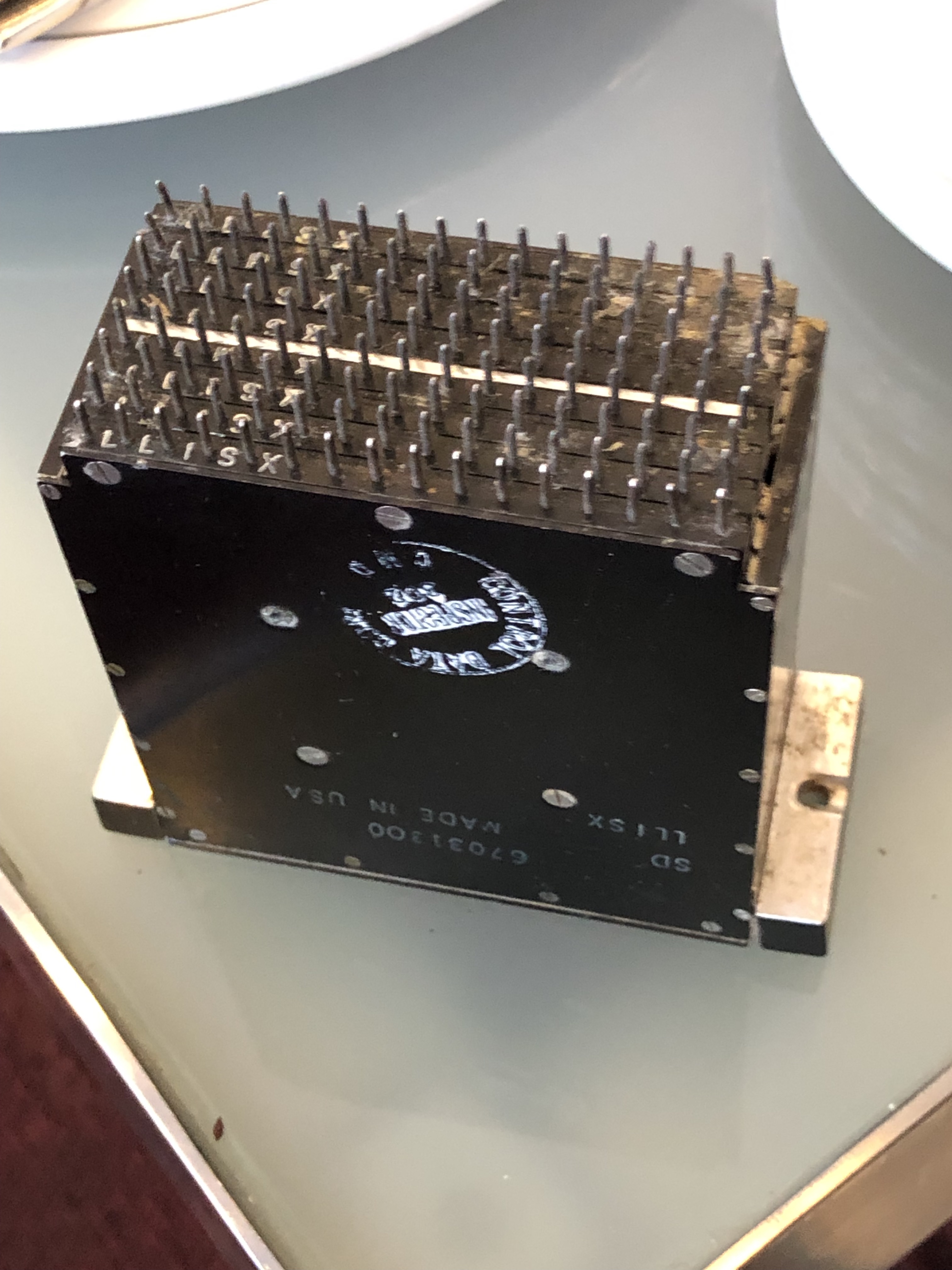
30. John Morrissey (ex-Csironet) holds a module from the CSIRO DCR CDC Cyber 76 processor. Here are two pictures:

31. Here is a montage of programming tools from the 1970s and 1980s:
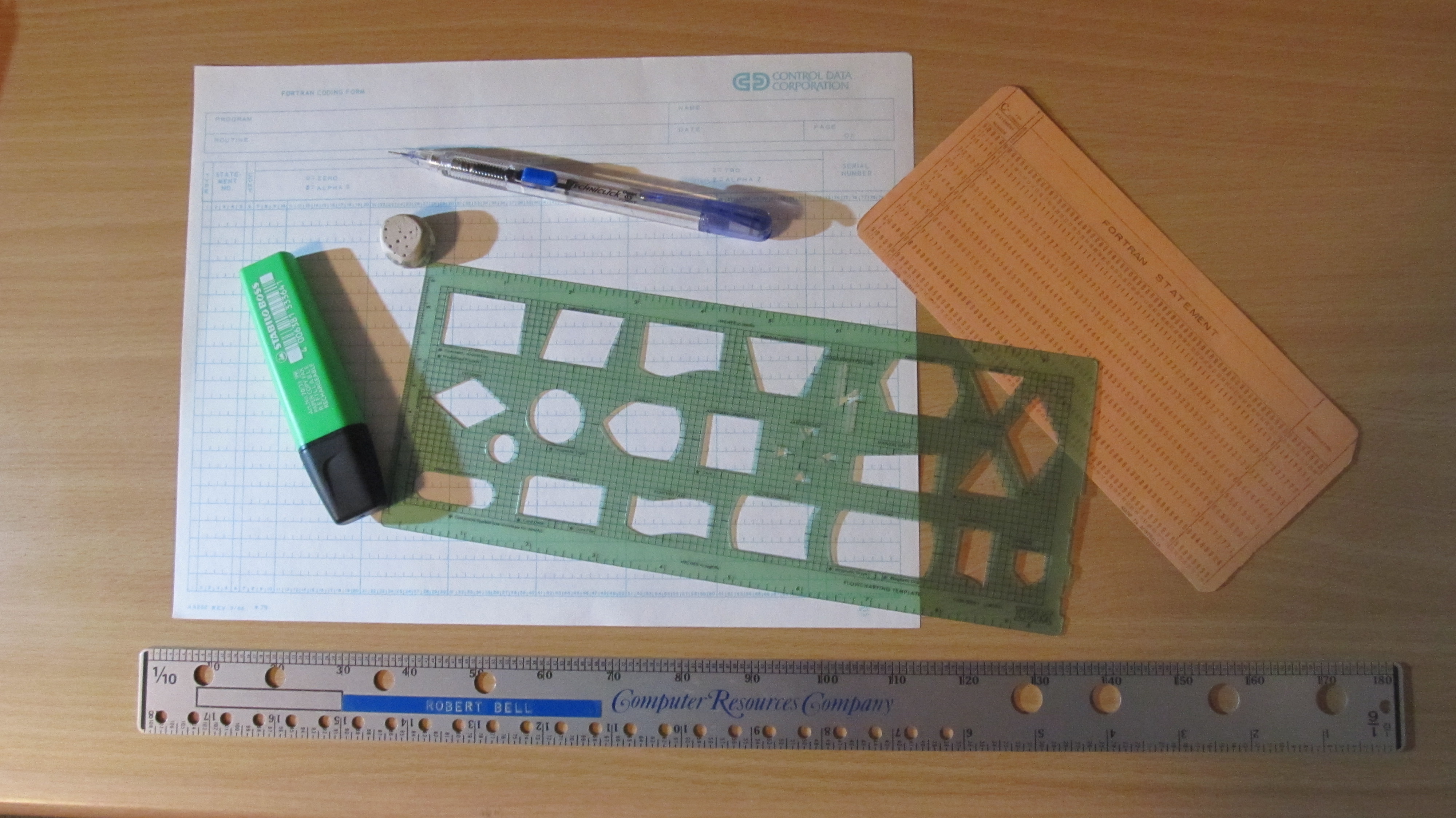
This shows:
- a coding form: programs were written on such forms, and then transferred to cards by the author or by a ‘punch girl’ – apologies, but that was the term used, I’m afraid. This particular one was a CDC Fortran – the rigid column-limited form of old Fortran is evident.
(C in column 1 for a comment, columns 1-5 for statement numbers, column 6 for a continuation flag, columns 7-72 for statements, and columns 73-80 for sequence numbers (rarely used in the CSIRO environment). - an automatic pencil – these followed on from clutch pencils and conventional pencils, and were a considerable (?) saving in that they were fine enough not to need sharpening.
- an eraser – most people coded in pencil, as mistakes were common. Tony Davies at Aspendale used to code using a fountain pen.
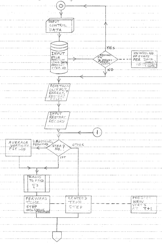
- a flow-chart template – flow charts were on the way out by the 1970s, as structured programming became the rallying cry for software development processes. “GOTOs were considered harmful!” Here is the first page from a flowchart from 1974.
- a punched card – this one is a Fortran one, and fairly unusual as being full-coloured – a plain buff colour was more common.
- a highlighter pen – these came into use around the end of the 1970s. Most output was on 11″ by 15″ paper, and a highlighter pen was ideal for highlighting important information or errors without obscuring the print.
- a special ruler, primarily for counting character positions on printed output. Output was printed 10 characters per inch horizontally, and 6 characters per inch vertically, and the ruler provided a quick way to determine the position of a character relative to the start of a line on a page without having to count each character. The ruler saved a lot of effort when trying to set up output using pre-Fortran 77 format statements:
98    FORMAT(29H OPTIMUM RELAXATION FACTOR = ,1PE18.11,24H  RESIDUAL MUL

     $TIPLIER = ,1PE18.11)
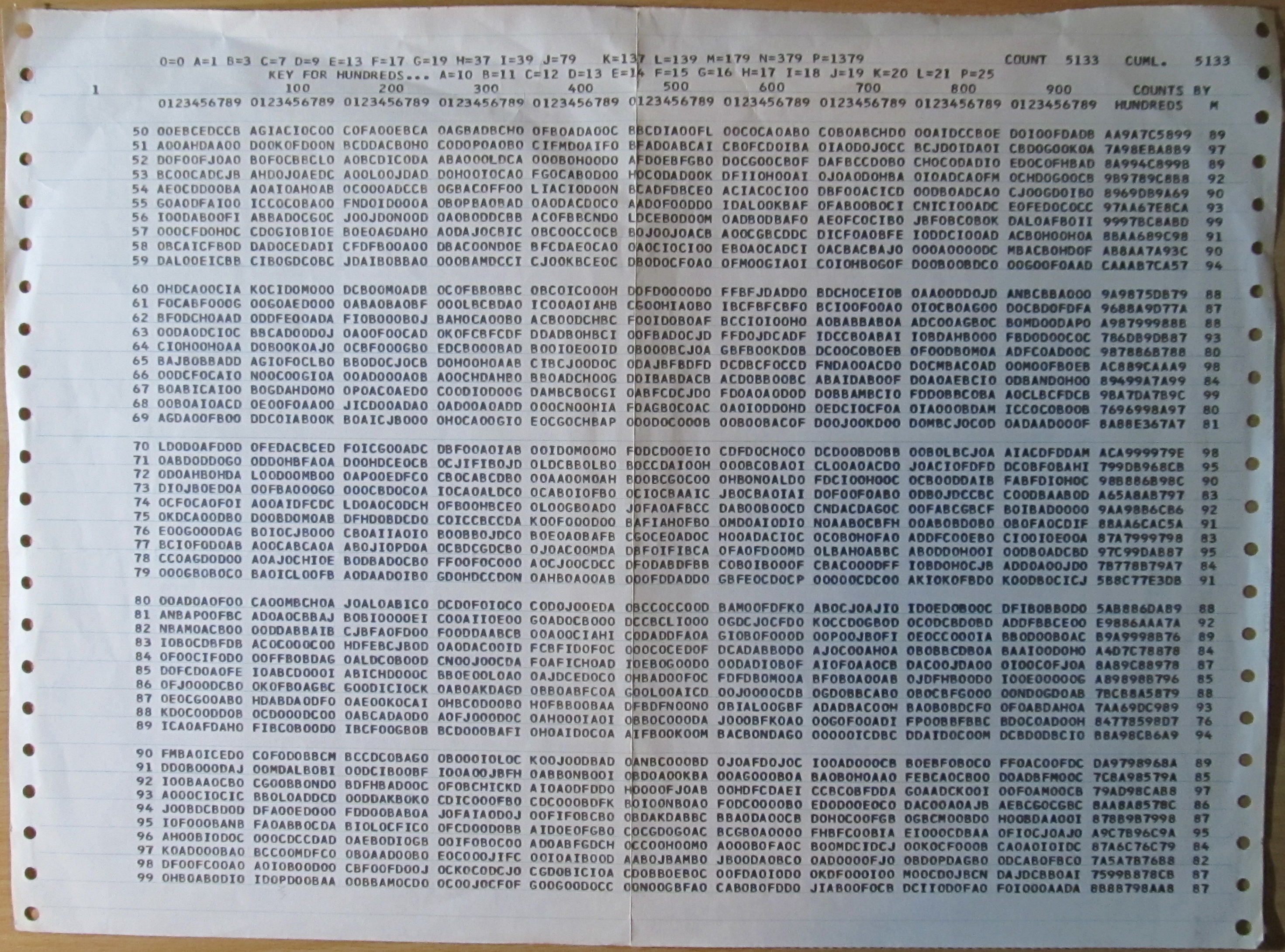
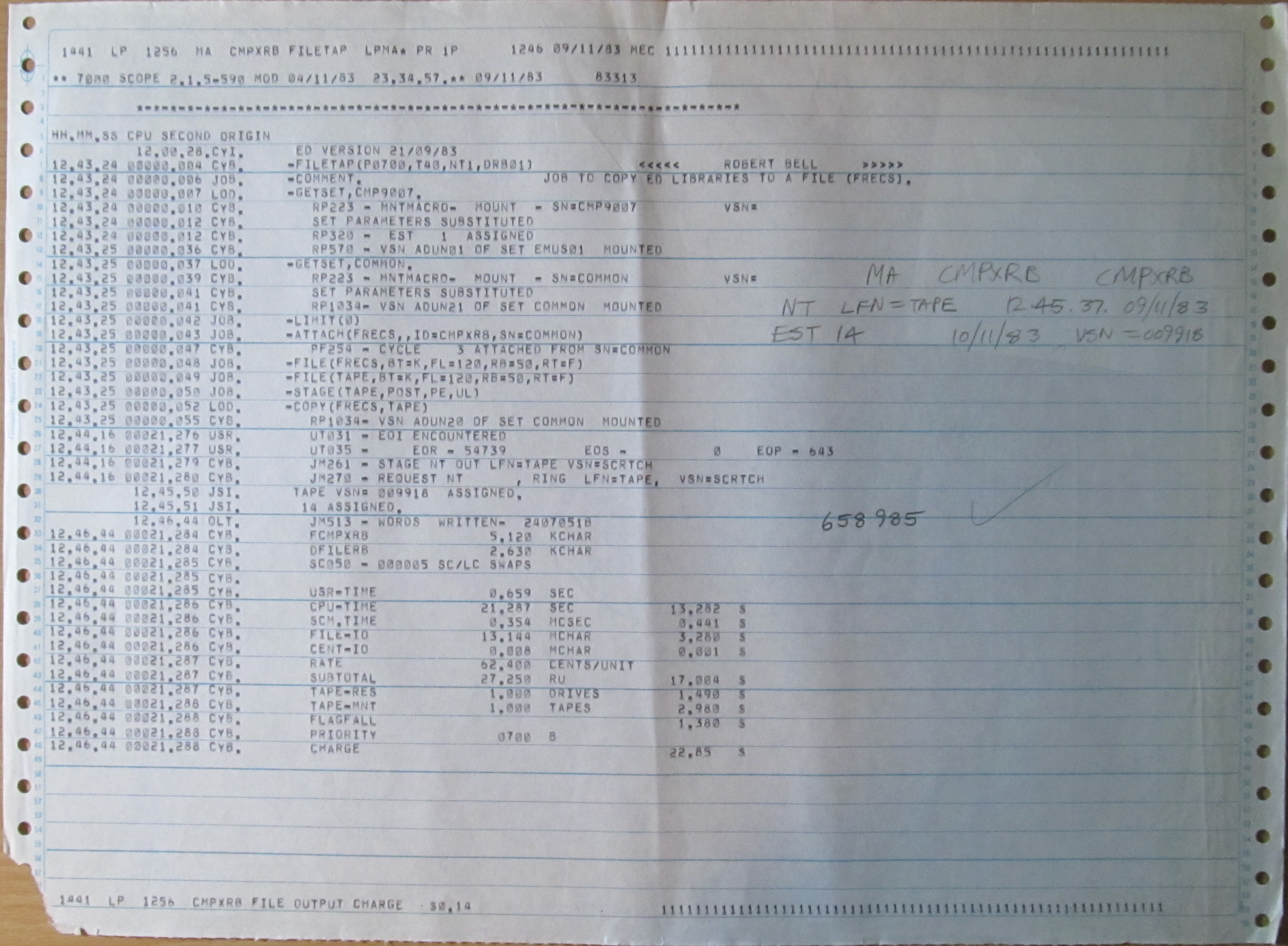
32. Here are some examples of pages of output (“printout”) on 11” x 15” fanfold sprocketed paper as used in line printers
a) Two pages showing a table of prime numbers to 100 000. I think this was produced on a CDC 3400 undergoing acceptance testing for DSD in about 1965, and has a clever encoding scheme (see the key at the top of the second page).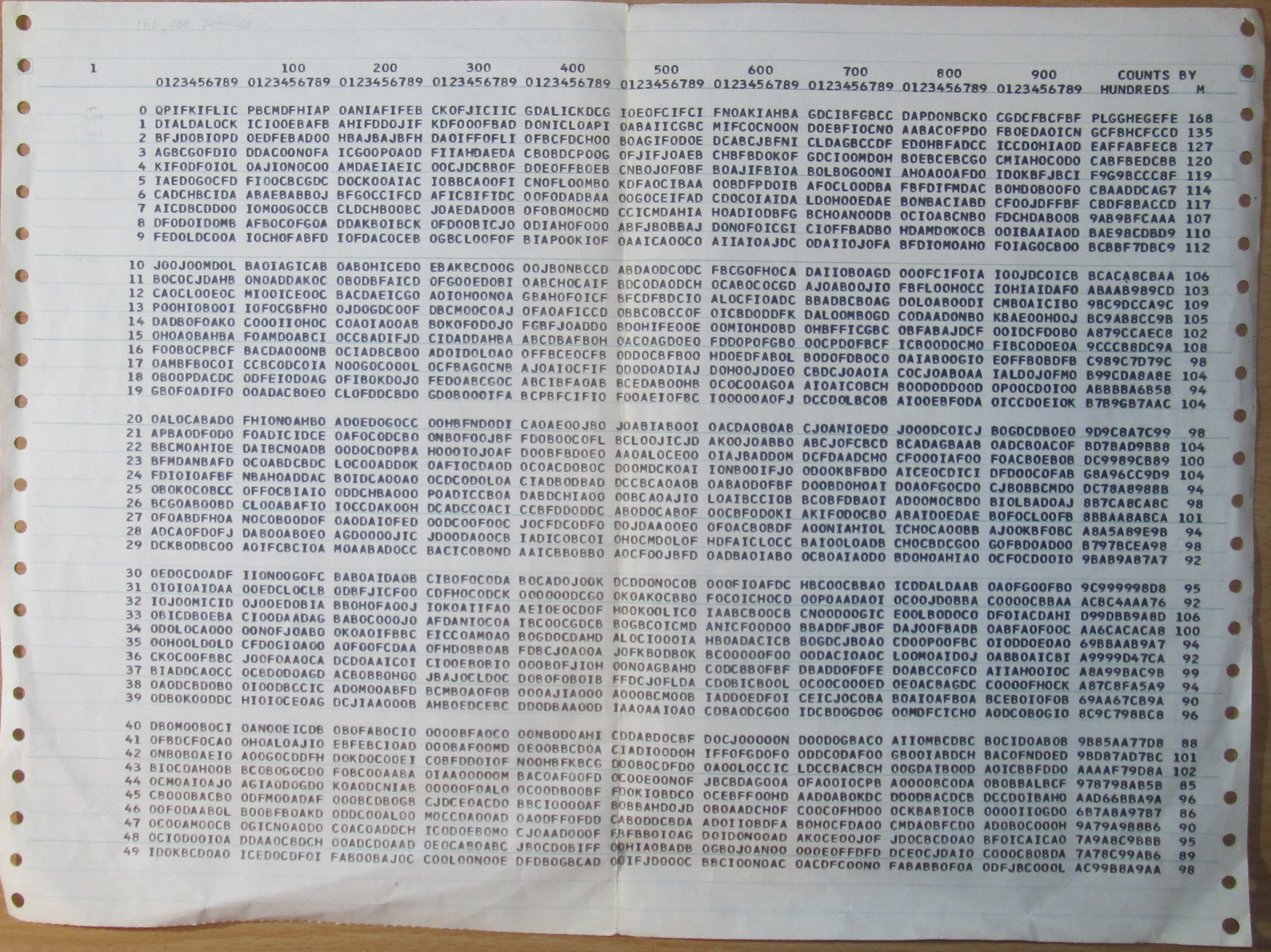
b) A listing of numbers, with a line-printer graph beside it. This was run on the Monash CDC 3200 in 1969.
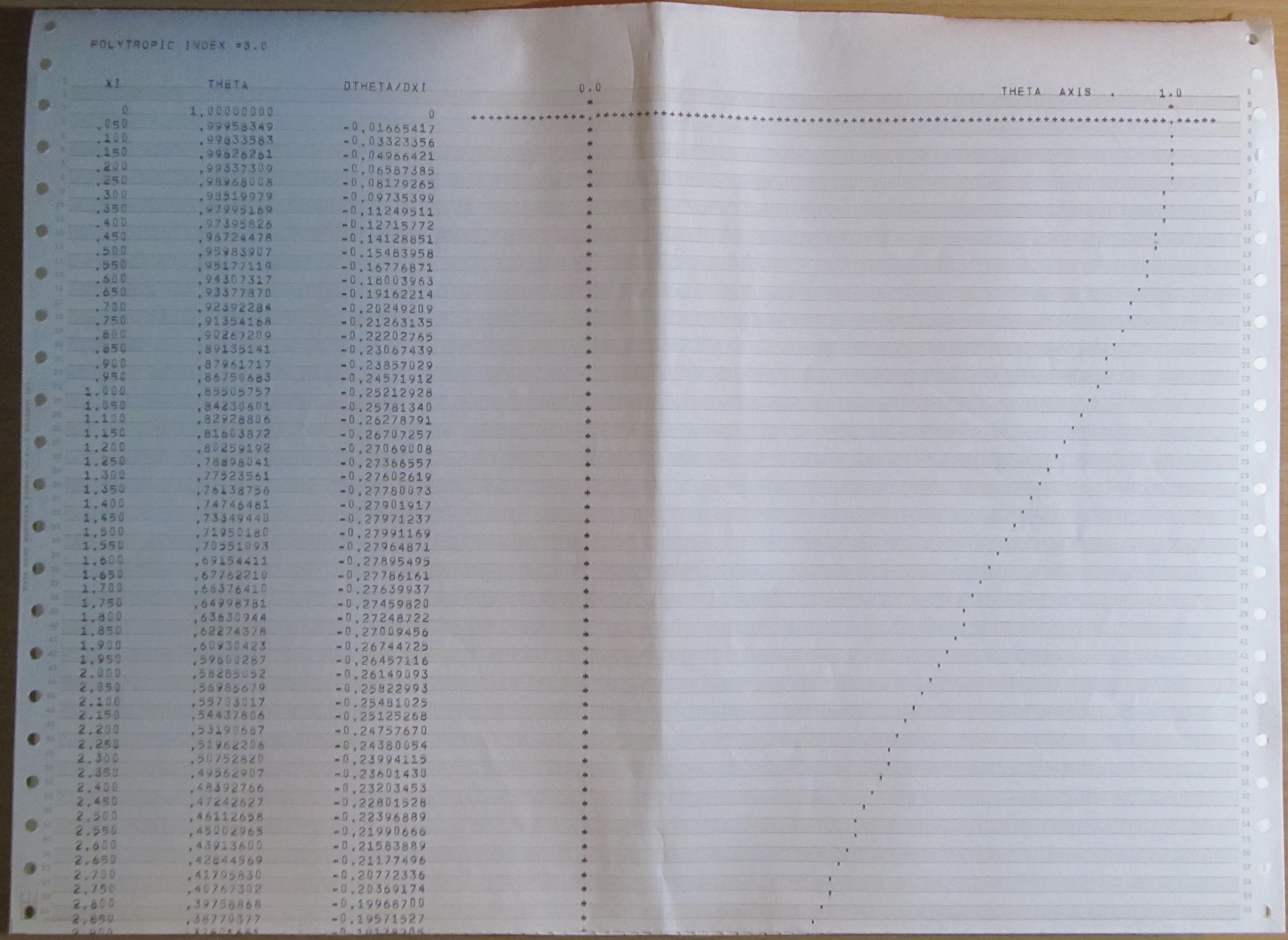
c) A sample output from the Cyber 76, in 1983. This particular job wrote fixed length records of source code to tape for transport to another site running an IBM mainframe. SCOPE2 job output started with a dayfile, which gave a summary of all the commands executed and the results of running the commands, with time stamps and running totals of CPU time used. Also included was a detailed summary of the charges!
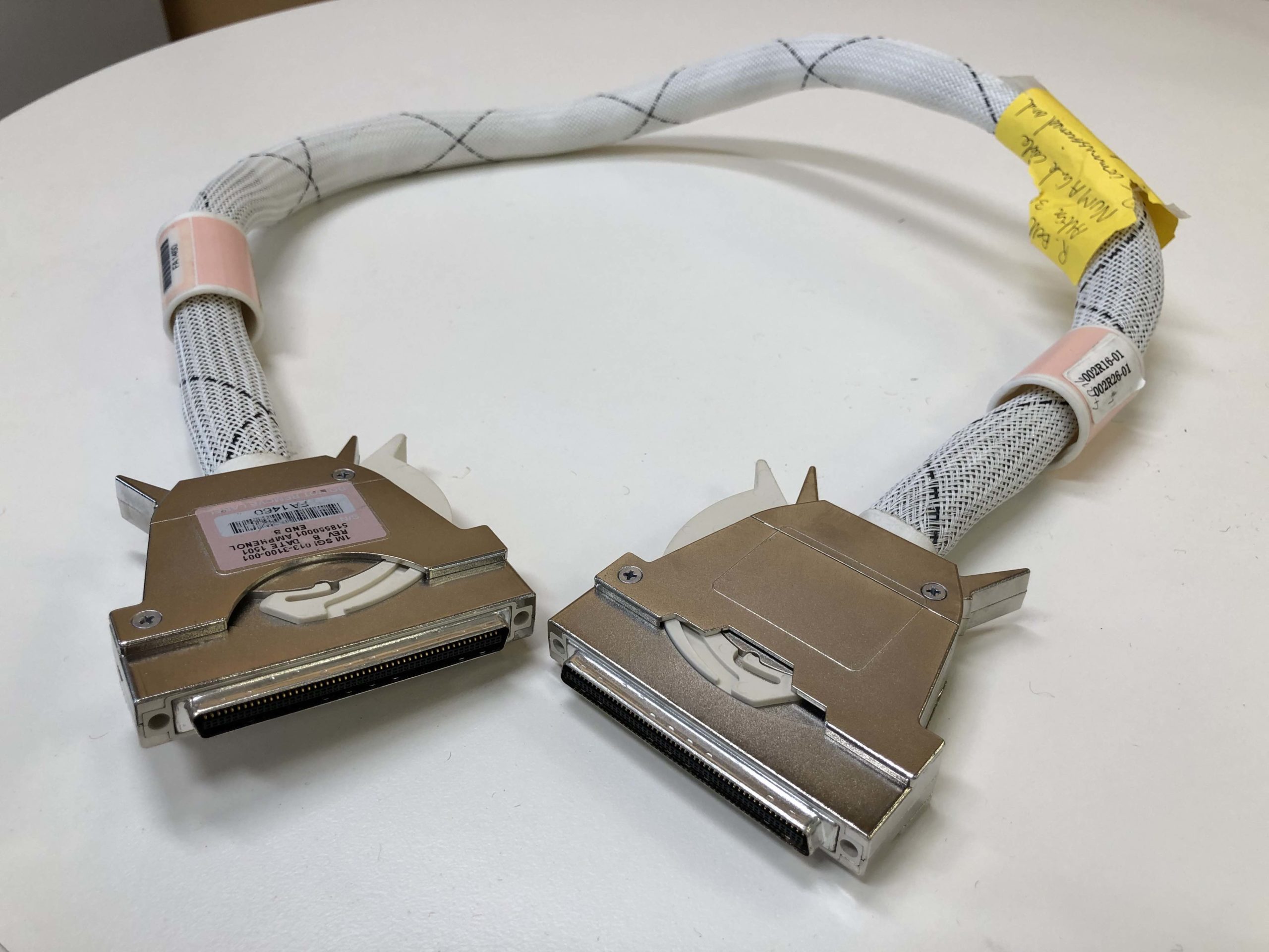
33. NUMAlink cable
CSIRO had a series of SGI large shared-memory systems from 2004 onwards. These were multi-node systems, like a cluster, but had a unified memory, and ran only one copy of the operating system, unlike a cluster. A NUMAlink system allowed for each processor to access all the memory, accomplished by cables such as the below linking all the processors and memory, so that the delays in accessing remote memory were tolerable. The picture below shows a NUMAlink cable from the SGI Altix 3700, which was installed in February 2004 and decommissioned on 2008-10-16. I counted 50 pins in a connector.
 34. The NEC SX series
The HPCCC had an SX-4, two SX-5s and a 28-node SX-6 system from 1997 to about 2011.
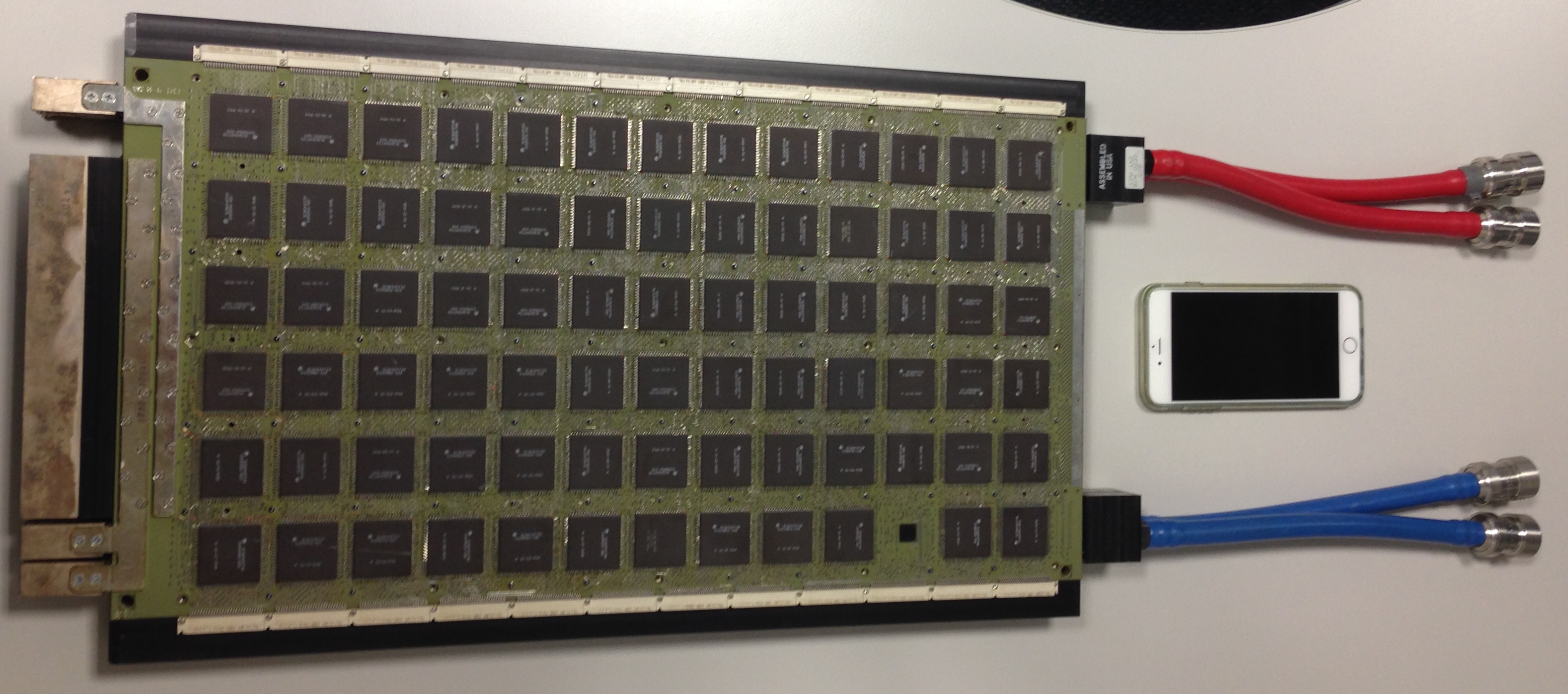
The SX-5s had 16 vector and scalar processors, and 128 Gbyte of memory. The memory was divided in 32,768 banks, to allow high speed vector access. Below is a photo of one memory module, containing 256 Mbyte of the 128 Gbyte total. There were 32 memory units, each with 16 modules. The memory technology was 47 ns SDRAM. Note the large number of connector points. Obtained 2004-06-02.
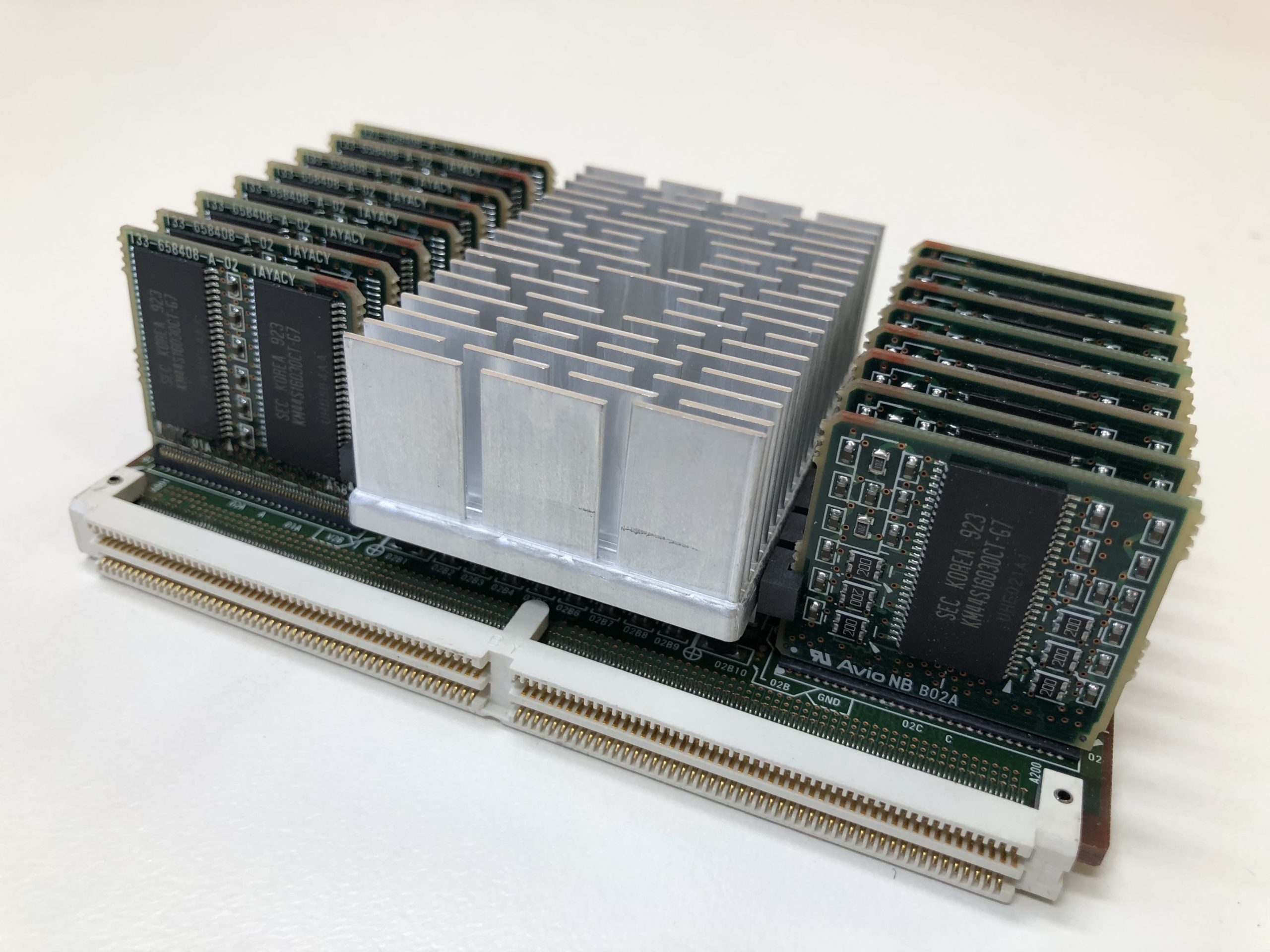
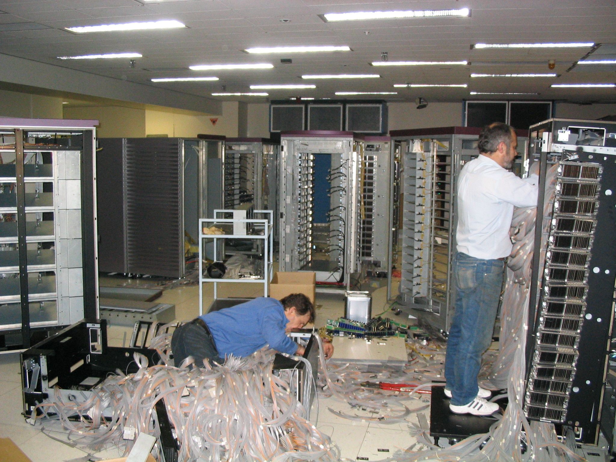
This amounted to a lot of wires – we estimated at least 16 x 32768 = 524 288 wires for the processor to memory connections: when the SX-5s were decommissioned, the engineers saw the full extent of the wiring – we estimated around 380 km. Here are some photos, showing Jack Dutkiewicz and Colin Paisley at work.

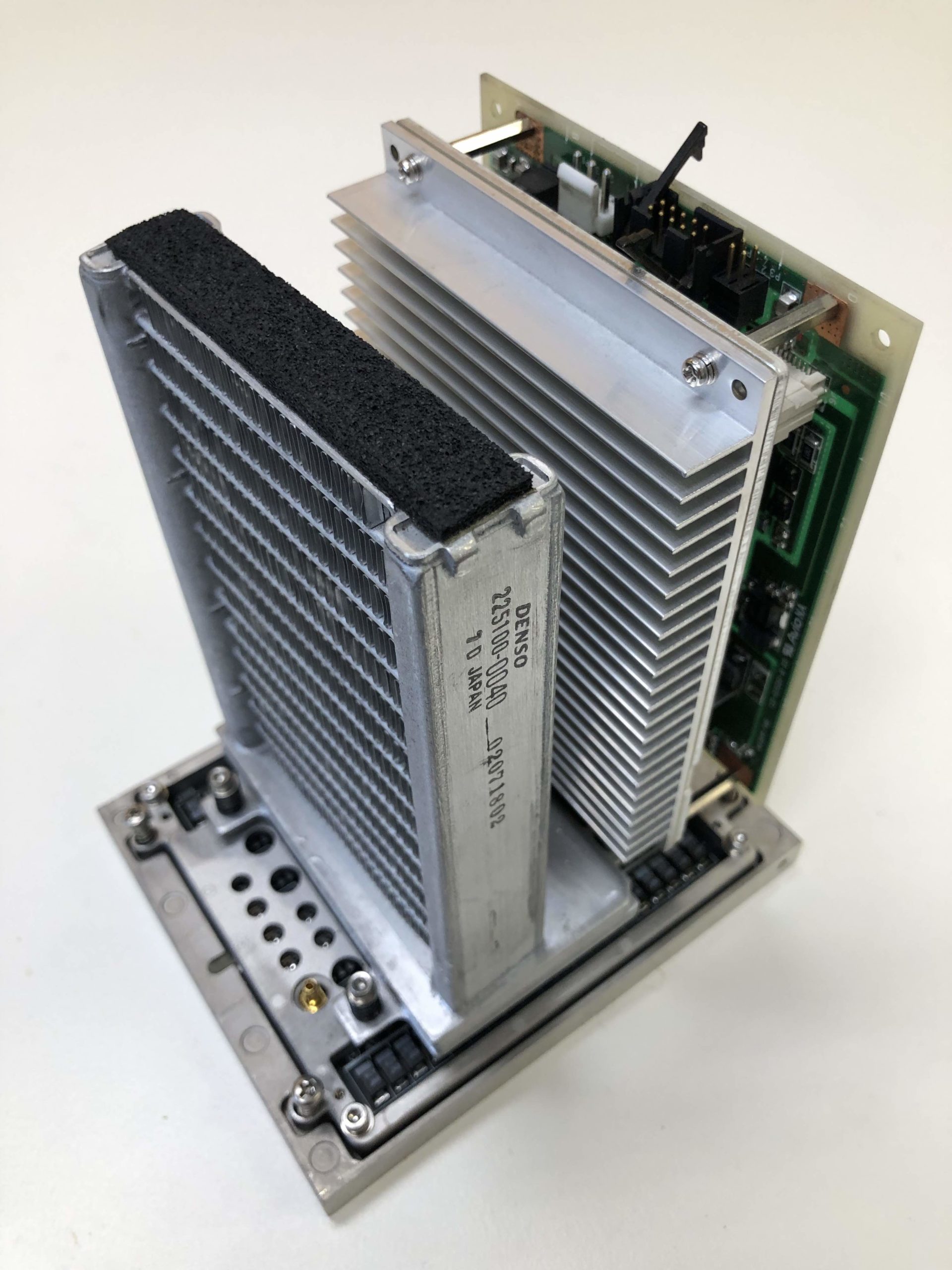
The SX-6 was based on the Earth Simulator System, with the vector CPU shrunk down to a single chip. The picture below shows the SX-6 CPU module: most obvious is the car-radiator technology used to cool it!
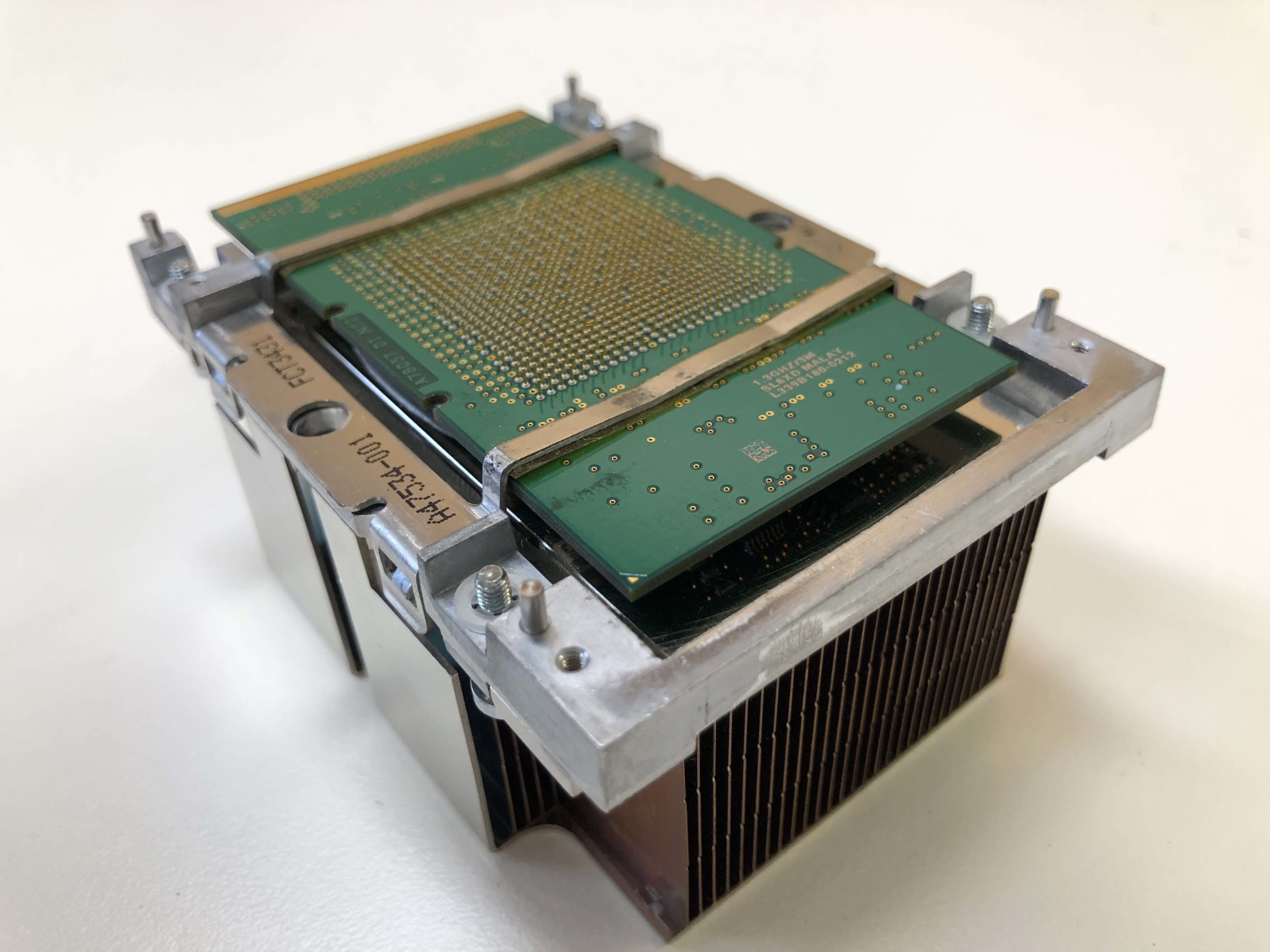
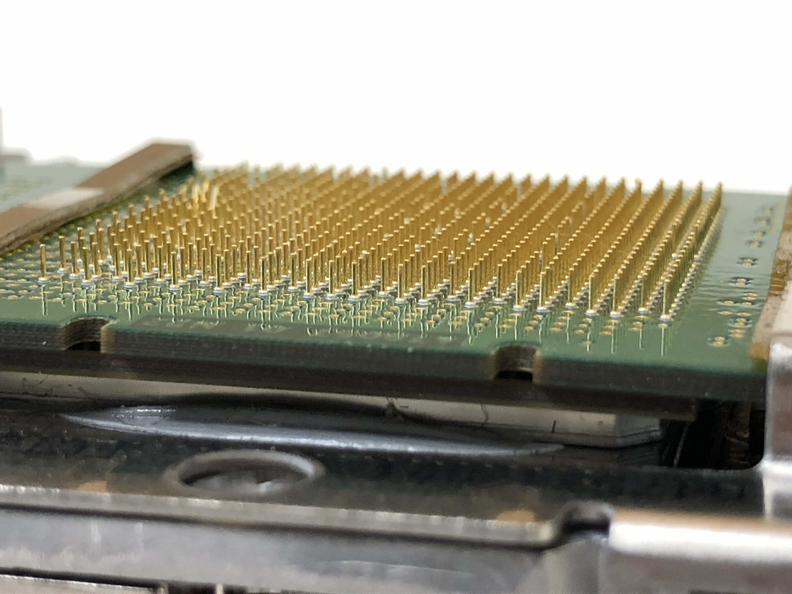
Here’s another module from this era, probably from the SX-6 front-end TX7 system which had Itanium processors. There are many copper cooling plates, and an array of gold pins (some of which are bent!).
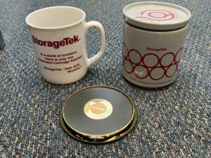
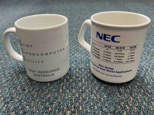
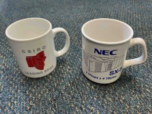
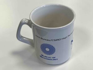
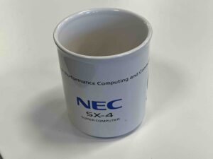
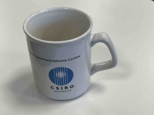
Computer vendors often produced souvenirs of their systemss, e.g. caps, and site-specific coffee mugs. Here are some pictures.
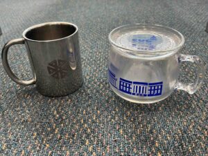
Finally, here is picture of a glass from Cray Research – the glass base was shaped to be reminiscent of the shape of the early Crays, with a bench seat.

Glass with bulbous base,
Holdings locations
Some of the artefacts and publications are held by Rob Bell at Clayton. Some are held under his desk at http://w3w.co/older.after.sticks (box C11), and some are in the basement of Building 001 – IT Build room archive area. Archive boxes series A and B are held in the IT Build room archive area, while series C boxes are in the Records store in building 001, room RCB.02.
Copies of publications, HPCbulls, brochures, annual reports, books, etc are held in the office near his desk.
SC Circulars can be seen by CSIRO staff at https://confluence.csiro.au/display/SC/SC+Circular
HPCbulls can be seen by CSIRO staff at https://confluence.csiro.au/display/SC/HPC+Bulletins .
A list of the contents of Rob Bell’s archive boxes can be seen by CSIRO staff at https://hpc.csiro.au/users/70294/records.1
Files from Csironet can be found by registered CSIRO users at /datastore/bel107/Csironet
Files from the CSIRO Cray Research UNICOS era (1990-2004) can be found by registered CSIRO users at /datastore/bel107/UNICOS
Files from accounting processes can be found by IMT SC staff at /datastore/asc/share/Accounting
Files related to this history can be found by IMT SC staff at /datastore/asc/share/Computer.History and /datastore/asc/Computing.History and /datastore/bel107/Computer.History .